
Custom Cell Format in Excel: How to Display Negative Values with Parentheses
Excel is a powerful tool for managing and presenting data, and one of its lesser-known features is the ability to customize cell formats. In this blog post, we’ll dive into the custom cell format “#,##0.00;(#,##0.00)” and explore how it can be used to display negative values with parentheses.
Understanding the Custom Cell Format
Before we delve into its practical applications, let’s break down the custom cell format “#,##0.00;(#,##0.00)”.
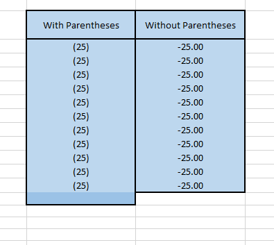
- Positive Values (#,##0.00): The format before the semicolon defines how positive values should be displayed. In this case, it specifies that numbers should be formatted with a comma as a thousand separator, two decimal places, and no parentheses.
- Negative Values ( ;(#,##0.00)): The format after the semicolon is for negative values. It tells Excel to display negative numbers within parentheses, following the same thousands separator and decimal places formatting.
Use Cases for the Custom Cell Format
Now that we understand the format, let’s explore some practical use cases for “#,##0.00;(#,##0.00)” in Excel:
1. Financial Statements: When creating financial statements or reports in Excel, it’s common to use parentheses to indicate negative numbers. This format makes the presentation of financial data cleaner and more intuitive. For example, if you have expenses or losses, they will be shown in parentheses, signifying a decrease in value.
2. Budgeting and Forecasting: In budgeting and forecasting spreadsheets, using parentheses for negative values enhances clarity. It makes it easier to distinguish between income and expenses, allowing stakeholders to quickly grasp financial insights.
3. Data Visualization: When building charts and graphs, the custom cell format can be applied to ensure that negative values in your data are clearly represented. This can be especially helpful in bar charts, pie charts, and other visualizations.
4. Invoice and Billing Documents: In Excel templates for invoices or billing documents, using parentheses for negative amounts is an industry-standard practice. It simplifies the reading of invoices by highlighting charges and credits effectively.
5. Dashboards and Reports: If you’re creating interactive dashboards or detailed reports, this format can be applied to maintain consistency in how numbers are displayed, improving the overall user experience.
Applying the Custom Format in Excel
To apply the “#,##0.00;(#,##0.00)” custom format in Excel, follow these steps:
- Select the cells or range of cells containing the numbers you want to format.
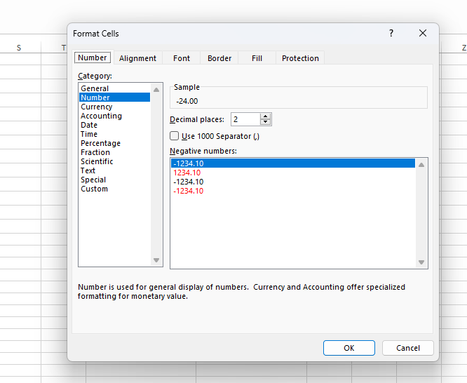
- Right-click and choose “Format Cells” from the context menu.
- In the Format Cells dialog box, go to the “Number” tab.
- Select “Custom” from the category list on the left.
- In the “Type” field, enter “#,##0.00;(#,##0.00)” as the custom format code.
- Click “OK” to apply the format to your selected cells.
Select the cells or range of cells containing the numbers you want to format.

Right-click and choose “Format Cells” from the context menu.

In the Format Cells dialog box, go to the “Number” tab.
Select “Custom” from the category list on the left.

In the “Type” field, enter
"#,##0.00;(#,##0.00)"as the custom format code.

Click “OK” to apply the format to your selected cells.

Voila! Your positive values will appear as usual, and negative values will be enclosed in parentheses.
In conclusion, the custom cell format “#,##0.00;(#,##0.00)” in Excel is a valuable tool for enhancing the presentation of data, especially in financial and data visualization contexts. By applying this format, you can make your spreadsheets more visually appealing and user-friendly while ensuring that negative values are easily distinguishable. Give it a try in your next Excel project and experience the difference it can make in data clarity and presentation.

Leave a Reply to prodentim review Cancel reply